03c Suggest ROIs (clustering-based, deprecated)

The ROI suggestion tool searches for bright or structured image regions that can be useful seed candidates. It is a separate workflow that runs before seed building — its output is just a set of ROIs, which then feed into the normal seed flow described in Seeds, spectra, and W maps.

The method runs in two stages. First it builds a 2D response map by collapsing the spectral stack and enhancing local bright structures. Then it groups the spatial candidates by spectral similarity so distinct component types get separate ROIs instead of being collapsed into one.

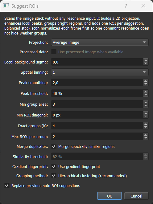
The dialog scans the current image stack without requiring resonance positions or reference spectra.

Settings reference

Setting	What it controls	Default	Practical effect
Projection	How the spectral stack is collapsed into one 2D response image.	Average image	See projection modes below.
Processed data	Whether the processed/background-subtracted stack is used when available.	Off	Enable if subtraction reveals the structures you want better than the raw stack. Disabled when no processed data are available.
Local background sigma	Size of the blurred background estimate subtracted from the projection.	8 px	Increase to suppress broad illumination gradients. Lower if real broad structures are suppressed.
Spatial binning	Downsampling before peak finding.	1×	Higher binning is faster and more robust against pixel noise, but can miss very small structures.
Peak smoothing	Gaussian smoothing applied to the response map before candidate detection.	σ = 1	Increase to suppress noisy speckles. Decrease to keep sharp or small structures.
Peak threshold	Required brightness relative to the response map.	0.65	Lower finds more and weaker regions. Higher keeps only the strongest candidates.
Min group area	Smallest connected bright region accepted as a candidate (pixels in binned projection).	3 px²	Increase to reject detector noise or isolated hot pixels.
Min ROI diagonal	Minimum size of the final ROI box in pixels.	0 px	Use to discard very small artefact ROIs. 0 px disables this filter.
Max suggested groups	Maximum number of distinct spectral groups to create in one run. Also sets the cluster count for hierarchical grouping.	3	Set slightly higher than the number of expected components to give the algorithm room to find all of them.
Max ROIs per group	Maximum number of spatial ROIs kept per spectral group.	1	Increase when multiple examples of the same component are useful for averaging.
Merge duplicates	Whether regions with very similar mean spectra are merged into one component group.	On	Keep enabled so the suggester does not fill the table with copies of the same spectral class.
Similarity threshold	Spectral similarity cutoff used only in greedy grouping mode. Has no effect when hierarchical grouping is on.	0.82	Higher merges fewer regions. Lower merges more aggressively. Only tune this when hierarchical grouping is disabled.
Gradient fingerprint	Augments the spectral fingerprint with the spectral derivative before similarity is computed.	On	Helps separate components that share a dominant peak but differ in slope, shoulder, or tail. See explanation below.
Hierarchical grouping	Uses Ward hierarchical clustering to force exactly k groups from the candidate pool instead of merging greedily by threshold.	On	More reliable when components are spectrally similar. Greedy mode (off) can be used when the number of distinct components is uncertain.
Replace previous auto ROI suggestions	Removes only earlier auto-suggested ROIs before creating new suggestions.	On	Keep enabled while tuning settings. Disable to accumulate batches without removing earlier suggestions.

Gradient fingerprint - how it works and why it matters

When two spectra are compared, the default measure is cosine similarity on raw intensity: it asks how much the two intensity traces point in the same direction. This works well for spectra that look fundamentally different. But for closely related variants — such as a lipid and a slightly modified lipid — both spectra might share a large, dominant peak at the same position. The raw intensity comparison sees that shared peak and reports 85–95% similarity, even though the two components differ meaningfully in the slope leading up to the peak, the steepness of the descent, or the presence of a small shoulder.

The gradient fingerprint adds a second channel of information by also comparing how the spectrum changes across channels — its first derivative. Intuitively:

• Two spectra with the same dominant peak but different rising edges will have very different derivatives near that peak.
• A shoulder that is invisible as a bump in intensity becomes a clear local maximum in the derivative trace.
• A broad flat peak and a sharper narrower peak can look almost identical in intensity but have very different curvature profiles.

Concretely, the algorithm computes the derivative trace, normalises both the intensity part and the derivative part independently (so neither dominates), and concatenates them into one combined fingerprint vector that is twice as long as the original spectrum. All similarity comparisons and clustering distances are then computed on this combined vector.

The result: two components that differ only in spectral shape details — not in peak position — become more distinguishable. In tests on synthetic bead data with five closely related lipid/protein variants (pairwise cosine similarities of 0.85–0.95 on raw intensity), enabling the gradient fingerprint improved separation from 2 to 3–4 detected components out of 5.

When to turn it off: - Spectra that are extremely smooth or consist of a single featureless broad peak have almost no derivative structure. The gradient channel adds only noise in that case. - Very noisy spectra (low SNR) where the derivative amplifies noise faster than it reveals real shape differences. In that case, increase Peak smoothing first.

Interaction with the similarity threshold: the gradient fingerprint changes what the fingerprint vector is, but the threshold and clustering operate on that fingerprint regardless. In hierarchical mode (default) the threshold is not used at all — the Ward clustering works from pairwise distances on the gradient-augmented fingerprints. In greedy mode, the threshold is compared against cosine similarity on the gradient-augmented fingerprints, so a gradient fingerprint effectively makes the threshold stricter: two spectra that were 88% similar on raw intensity might be only 80% similar once the gradient differences are included.

Projection modes

Balanced stack scan (recommended starting point) Each spectral channel is independently normalized before being combined into the projection. This prevents one dominant resonance from overwhelming weaker ones, so all components get a fair chance to appear in the response map.

Multi-band scan The stack is split into several spectral bands and each band is projected independently. Candidates from all bands are then merged while suppressing spatial duplicates.

Use this when your data spans a wide spectral range and contains many distinct resonances that are spread across separate regions of that range — for example, a CARS stack that covers both the fingerprint region (1000–1800 cm⁻¹) and the CH-stretch region (2800–3100 cm⁻¹) at the same time. In that case a single projection — even a balanced one — still collapses the whole spectrum into one image, and components that are only bright in one narrow band can get buried by activity from other bands. Multi-band scan gives each spectral region its own independent projection pass, so components isolated to one region have a fair chance of being detected.

If your stack is narrower and all components share roughly the same spectral region, Balanced stack scan is sufficient and faster. Multi-band scan is slower and only pays off when resonances are genuinely distributed across multiple distinct spectral windows. Set Exact groups (k) to the total expected number of components across all bands combined.

Average image Simple mean of all channels. Faster. Biased toward structures that are bright across many channels. Good when all features are prominent and the stack has high SNR.

Maximum projection Keeps the brightest value across all channels at each pixel. Useful for locating any structure that is bright in at least one channel, but tends to over-detect in noisy stacks.

Current frame Uses only the currently displayed channel. Use for single-channel inspection or to seed a component known to be visible at one specific resonance.

Choosing settings for your data

Start with Average image and defaults. For most datasets this is sufficient — channels are typically in a comparable intensity range and the average gives a clean spatial contrast map. Switch to Balanced stack scan only if one channel dominates so strongly that weaker components disappear in the average.

If components are missed: - Increase Max suggested groups by 1–2 above the expected number of components. - Lower Peak threshold (try 0.25–0.35) to accept weaker candidates. - Reduce Peak smoothing (try σ = 1) if features are small or sharp. - Switch to Multi-band scan if missed components are known to be in a different spectral region than the detected ones.

If too many spurious suggestions appear: - Increase Peak threshold (try 0.50–0.60). - Increase Min group area (try 8–20 px²) to reject small noise artefacts. - Increase Spatial binning (try 2× or 4×) for very noisy data.

For spectrally similar components (e.g., closely related cell types, lipid subtypes): Keep Gradient fingerprint on. The gradient encodes slope and shoulder information that pure intensity cosine similarity cannot distinguish. Keep Hierarchical grouping on so that forced-k clustering separates the candidates instead of collapsing them by threshold.

Hierarchical grouping: all suggested ROIs look the same? Hierarchical clustering forces exactly k groups from whatever spatial candidates the first stage found. If all k groups end up representing the same component type, the candidate pool itself is too uniform — the dominant structure was simply detected k times in different spots. The fix is upstream: lower Peak threshold (try 0.25–0.35) so the spatial scan also picks up weaker, less prominent structures that may belong to other components. If those weaker structures are small or sharp, also reduce Peak smoothing (try σ = 1) so they are not blurred out before detection. With a more diverse candidate pool, the clustering has something real to separate.

For noisy data (low SNR, shot-noise dominated): Use Peak smoothing σ = 2 (default) or higher. A higher Spatial binning also helps. Increase Local background sigma if illumination is uneven.

For clean data with sharp, well-separated features: Peak smoothing σ = 1 often works better. The default σ = 2 may blur small features or merge nearby peaks.

The similarity threshold matters most in greedy mode. With Hierarchical grouping on (default), the algorithm forces exactly k clusters regardless of pairwise similarity, so the threshold has less influence. If you switch to greedy mode, lower the threshold (0.75–0.80) for closely related spectra and raise it (0.88–0.92) for clearly distinct ones.

Fundamental limitation: components whose spectra differ by less than ≈5–10% cosine distance (e.g., one spectrum is a near-linear combination of another) cannot be reliably separated by any spectral grouping method. In that case, draw ROIs manually in regions where one component is visually dominant.

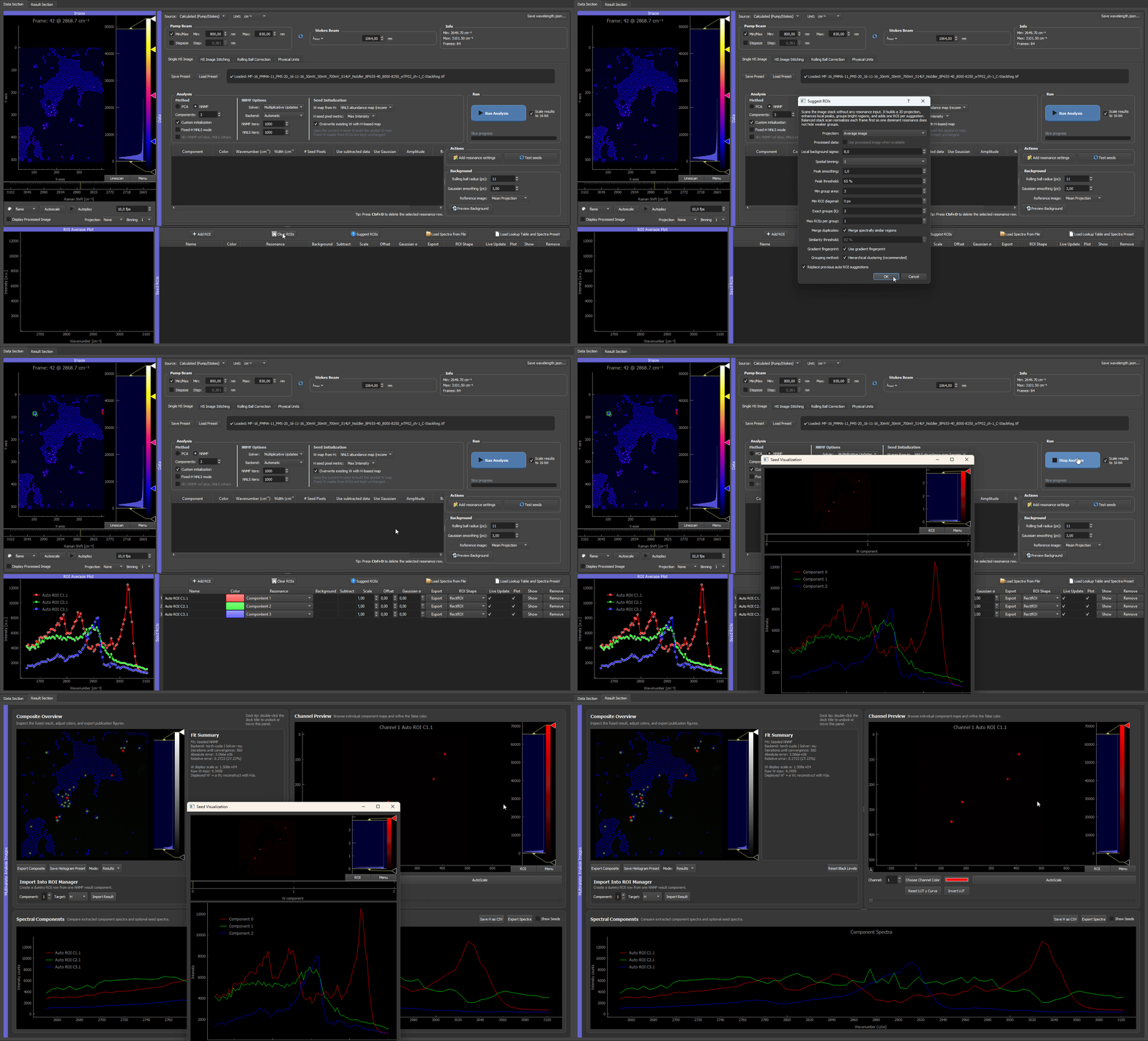
After suggestions are created, treat them like normal ROIs: move or resize them if needed, rename the rows, assign colors, check the ROI average spectra, and remove suggestions that are not useful seeds.

How the algorithm works internally

This section is for advanced users who want to understand what happens under the hood and why certain settings have the effect they do.

Stage 1 — Response map

The spectral stack (channels × height × width) is collapsed into one 2D response image depending on the chosen projection mode. In Balanced stack scan mode each channel is independently contrast-normalized before combining, and channels are averaged with weights proportional to their spatial variance — channels that carry more spatial structure contribute more. This prevents a single dominant resonance from drowning out weaker ones.

A blurred copy of the projection (radius controlled by Local background sigma) is then subtracted to suppress broad illumination gradients. The result is divided by the local standard deviation to normalize for local contrast variation. The final map therefore reflects relative local brightness rather than absolute intensity — a dim structure in a quiet region of the image can score just as highly as a bright structure in a bright region.

Stage 2 — Candidate extraction from the response map

Coarsen and smooth. The normalized map is downsampled by Spatial binning and then Gaussian-blurred by Peak smoothing. This suppresses pixel noise before any detection decisions are made and defines the spatial scale at which objects are expected.

Local maxima. A maximum filter marks every pixel that is the brightest in its local neighborhood. These become candidate peak locations.

Multi-threshold sweep. Rather than applying one fixed threshold, the algorithm sweeps across 8 levels from the user's Peak threshold down to roughly 8% of the map maximum. At each level a percentile floor also drops (from the 75th to the 15th percentile of positive values) to prevent the floor from suppressing detections in low-signal images. This sweep is why the algorithm can find both a dominant bright structure and a weaker structure that is 3–5× dimmer in the same run — the dominant structure is captured at the high threshold and the weaker one is picked up at a lower level.

Connected-component labeling. At each threshold level the thresholded map is segmented into connected blobs. Each blob is a candidate object. Blobs smaller than Min group area are discarded.

Peak-to-box refinement. Inside each blob the local maxima are ranked by brightness. For each peak a secondary threshold is applied at 72% of that peak's own value, carving out the tight bright core around it. The bounding box of that core becomes the proposed ROI box, padded outward by a few pixels.

IoU deduplication. Before accepting a box it is compared against all previously accepted boxes. If it overlaps an existing box by ≥ 60% (within the same blob) or ≥ 45% (across the whole sweep) it is discarded. This prevents the same structure being proposed repeatedly at different threshold levels.

Scale back. Boxes are scaled from the coarsened coordinate system back to the original image pixels, with padding added.

The output of this stage is a pool of spatial candidates ranked by peak brightness, capped at Exact groups × Max ROIs per group × pool factor.

Stage 3 — Spectral grouping

Each candidate ROI's mean spectrum is extracted and converted into a spectral fingerprint. With Gradient fingerprint on, the fingerprint is the concatenation of the unit-normalised spectrum and its unit-normalised first derivative, making shape differences (shoulders, slopes, tails) visible alongside peak positions.

Hierarchical grouping (default) applies Ward linkage clustering on the pairwise cosine distances between fingerprints and cuts the resulting tree at exactly k clusters, where k = Exact groups. This forces separation even between candidates that are spectrally similar, which greedy threshold merging would collapse into one group.

Greedy grouping (hierarchical off) instead walks the ranked candidate list and merges each new candidate into the most similar existing group if the cosine similarity exceeds the Similarity threshold, otherwise starting a new group.

Where the algorithm works well and where it does not

The spatial stage is reliable for isolated compact objects — beads, nuclei, cells, labelled structures — where different component types occupy different spatial positions in the image.

It cannot separate spatially overlapping components. If two materials are mixed within the same pixel region the spatial stage sees one blob, and only the spectral grouping stage can try to resolve the difference. If those two materials are also spectrally very similar (cosine similarity ≥ 0.90), no grouping method can reliably distinguish them automatically — manual ROI placement in regions where one material dominates is the only reliable path.

Very large structures that fill most of the image may be suppressed by the local background subtraction step. And if the dominant structure is so bright that the threshold sweep fills its entire candidate quota before reaching lower thresholds, weaker structures will not appear in the pool at all — lower the Peak threshold or increase Exact groups to give the sweep more room.