Concepts
This page explains the scientific and algorithmic ideas behind the GUI. It is intended as background reading. For practical mode selection, see Analysis modes. For the full mathematical treatment, see NNMF and NNLS modes.
Hyperspectral Image Stacks
A hyperspectral image is a 3D array:
channel × height × width
Each frame along the channel axis is a grayscale image recorded at one spectral position. Stacking all frames gives a datacube where every pixel has a full spectrum.
In coherent Raman scattering (CRS/CARS/SRS) microscopy, the spectral axis corresponds to Raman shift values, and each frame shows the sample at one vibrational resonance frequency. In fluorescence microscopy, the axis may correspond to emission wavelengths or named fluorophore channels.
The challenge with hyperspectral data is that looking at dozens of frames one by one is slow and often ambiguous, especially when:
- signals overlap spectrally (two resonances contribute to the same channel),
- background varies spatially and spectrally,
- the signal-to-noise ratio is low.
Multivariate analysis addresses this by summarizing the whole stack as a small set of component maps and spectra.
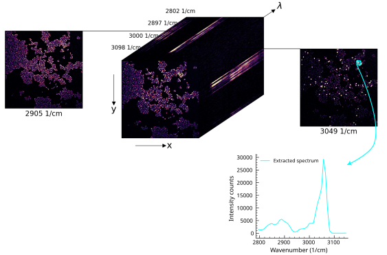
3D hyperspectral CARS microbead mixture bead data cube. Each channel is a grayscale image at one Raman shift. Different spectral properties are making the beads distinguishable as illustrated by the extracted PS bead spectrum from the ROI (cyan)
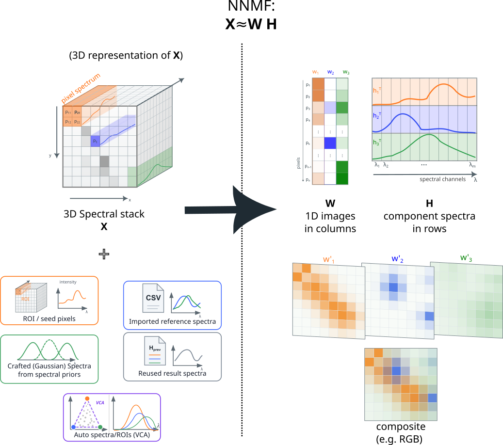
The Unmixing Model: X ≈ WH
The core idea is that each pixel spectrum can be approximated as a weighted sum of a few basis spectra:
In matrix form for all pixels at once:
The one equation behind every analysis mode
All four modes (PCA, random NNMF, seeded NNMF, fixed-H NNLS) solve a variant of X ≈ WH. The differences are only what is held fixed and what constraint is applied. PCA allows signed values; the three NMF/NNLS modes enforce non-negativity. Random NNMF discovers both W and H; seeded NNMF starts from user-provided seeds and refines both; fixed-H NNLS locks H and solves only W. Internalizing this matrix picture is the single most important step for getting good results.
where:
- \(X\) is the data matrix, shape
(n_pixels, n_channels), - \(W\) is the spatial abundance matrix, shape
(n_pixels, n_components), - \(H\) is the spectral basis matrix, shape
(n_components, n_channels).
Each row of \(H\) is one component spectrum. Each column of \(W\) is one component's spatial map, reshaped into an image for display.
In the GUI: - component spectra (rows of \(H\)) appear in the spectral plot, - component maps (columns of \(W\)) appear as grayscale images and as layers in the composite, - the composite view fuses all component maps into a false-color image.
Spatial Maps W and Spectral Components H
W maps answer: where is this component present, and how strongly?
- A high value at a pixel means the corresponding component contributes a large fraction of the signal there.
- Component maps are non-negative abundance-like coefficients, not direct copies of raw detector values.
- After analysis, W values can exceed the original 16-bit range if the spectral basis is scaled in a particular way. This is expected.
H spectra answer: what does the signal look like when this component is present?
- Each H row is a spectral fingerprint or reference spectrum for one component.
- In seeded workflows, H is initialized from ROI spectra, loaded reference files, or Gaussian models.
- In fixed-H NNLS, H stays fixed and only W is solved.
The factorization has a per-component scale ambiguity: scaling the W column (image map) by a constant and the matching H row (spectrum) by its inverse leaves \(W H\) unchanged. The GUI therefore normalizes generated W seeds to a comparable unit maximum and leaves the spectral/count scale in the H seeds. In seeded NNMF the optimizer is free to undo this convention during fitting; the choice mainly avoids letting raw image-count differences dominate the initial W maps.
ROI-Derived H Seeds
ROIs (regions of interest) are rectangular regions drawn on the image. The mean pixel spectrum inside an ROI is used as an initial guess for the corresponding component spectrum.
This works well when: - different image regions are clearly dominated by different chemical components, - the ROI spectrum approximates the pure-component spectrum.
Multiple ROIs assigned to the same component are averaged, which can improve the seed estimate if no single region is spectrally pure.
Spectral Priors from Files or Gaussian Models
Spectra do not have to come from image ROIs. The GUI also accepts:
- Loaded spectra:
.txt,.asc, or.csvfiles with two columns (axis, intensity). Multi-column CSV files can load several spectra at once. - Gaussian resonance models: define a resonance center and half-width; the GUI generates a Gaussian-shaped spectrum for that component.
Loaded spectra are re-sampled to the current image spectral axis by linear interpolation before analysis. The seed actually used is therefore the interpolated spectrum, not the raw file data.
Gaussian models create a dummy ROI row for the relevant component and are useful when the approximate peak position and width of a resonance are known but no reference measurement is available.
W-Seed Estimation Modes
When only an H seed exists, the GUI has to estimate an initial W map before starting NNMF. Five modes are available:
| Mode | Behavior |
|---|---|
nnls |
Solves a non-negative least-squares fit against all seeded H spectra simultaneously. The most aggressive mode — aims at maximum unmixing, so pixels tend to be assigned to a single component. Best when chemistries are expected to live in different pixels. |
selective_score |
A heuristic spatial score based on the projection of the image onto the target spectrum, down-weighted where competing spectra score higher. Softer than nnls — does not force one winner per pixel. Prefer it when mixing across pixels is physically expected. |
h_weighted |
A legacy channel-weighted image heuristic. Less common in practice. |
average |
Uses the mean image across all channels. A simple uniform-energy fallback. |
empty |
A near-zero homogeneous map. Lets NNMF build the spatial structure entirely from scratch for that component. |
These modes only affect the initialization. In seeded NNMF, the optimizer then updates both W and H freely from the starting point.
Generated W seeds are normalized component by component for seeded NNMF initialization. This does not constrain the final NNMF scale, because the optimizer can rescale each W/H component pair during fitting by adjusting both W and the matching H row.
Seeded NNMF vs Fixed-H NNLS
The two main user-facing analysis modes differ in one important way:
Seeded NNMF: seeds are starting points. Both W and H are updated during fitting. The final result can differ from the seeds.
Fixed-H NNLS: the H matrix is locked to the provided seeds. Only W is fitted. The result maps are the best non-negative abundance coefficients for those fixed spectra.
Use seeded NNMF when you want the algorithm to adapt and refine the spectral estimates. Use fixed-H NNLS when the spectra are already trusted and must stay stable.
Which mode for which job?
- First look at an unknown sample → PCA or random NNMF.
- You have ROIs / reference spectra and want clean unmixing → seeded NNMF. This is the main publication-grade workflow.
- The spectra are already trusted and you want stable maps across slices / time points / FOVs → fixed-H NNLS. Strictest mode; most comparable results across 4D.
This distinction matters for scaling. In fixed-H NNLS, W is the fitted result, not just a starting seed. The usual NNMF scale ambiguity is no longer a free normalization choice: because H is fixed, rescaling W alone changes \(W H\) and therefore changes the reconstruction error. Preserving the same product would require inverse rescaling of H, which fixed-H mode deliberately does not allow. The internal W coefficients are therefore kept on the scale required to reconstruct \(X\) from the fixed H spectra. Display or export can still rescale maps for visualization, but the fixed-H NNLS fit itself should not normalize W to unit maximum.
4D z/Time Workflows
When data is 4D (z-stack or time series), the stack has an extra outer axis:
z_or_time × channel × height × width
The GUI can analyze each z/time slice independently using the same seed setup, which is useful for:
- tracking spectral changes over time,
- comparing different z planes with a common spectral basis,
- mapping the same components across a volumetric stack.
In fixed-H NNLS mode, the same spectral basis is applied to every slice, making the resulting W maps directly comparable. In seeded NNMF mode, the basis is re-initialized for each slice from the same seeds, so mild per-slice adaptation is possible.
 Fixed H NNLS result for a unmixed U2OS fluorescence z-stack. The resultuing H spectra are locked across slices.
A special option, fast multislice NNMF, uses NNMF on a reference slice and then NNLS for all other slices. This is faster than running full NNMF on every slice and keeps the spectral basis consistent across the series.
Non-Negativity Constraint
All analysis modes except PCA enforce non-negativity: both W and H (where applicable) contain only values ≥ 0. This constraint is physically motivated because:
- intensities and photon counts are non-negative,
- molecular concentrations are non-negative,
- the mixing model should be additive, not a cancellation of positive and negative contributions.
PCA does not enforce non-negativity and is therefore primarily a diagnostic tool rather than a physically interpretable decomposition.
Background Components
The analysis model allows one or more components to represent a broad, slowly varying background rather than a chemical species. This is not usually the first tool to try; it is most useful when the background is hard to detect with ordinary ROIs or when removing it as preprocessing would also remove real sample signal. Background components can be:
- drawn as spatial ROIs over background-dominated regions,
- generated as a W-only seed from a projected image (mean, max, or min projection),
- imported as a fixed W map from a previous result.
Having an explicit background component in the model can improve the separation of weak chemical components from a difficult baseline, but it should be treated as a modeling choice that needs inspection rather than a default correction step. This setting can help in particular when background is disturbing false color channels that carry specific information.
Scale Bars and Physical Units
The physical size of each pixel (in nm, µm, or mm) is tracked in the physical-units panel. This information is used for:
- scale bars overlaid in the GUI and in exported images,
- pixel-size metadata written into exported Fiji/ImageJ TIFFs.
After binning, stitching, or loading a preset, check that the pixel size still reflects the actual acquisition pixel size.