03b ROI Manager in detail
The ROI Manager is the central place where spatial ROIs, spectral seeds, fixed W seeds, labels, colors, and component assignments are organized. It is not only a drawing tool. It defines how the analysis interprets user input.
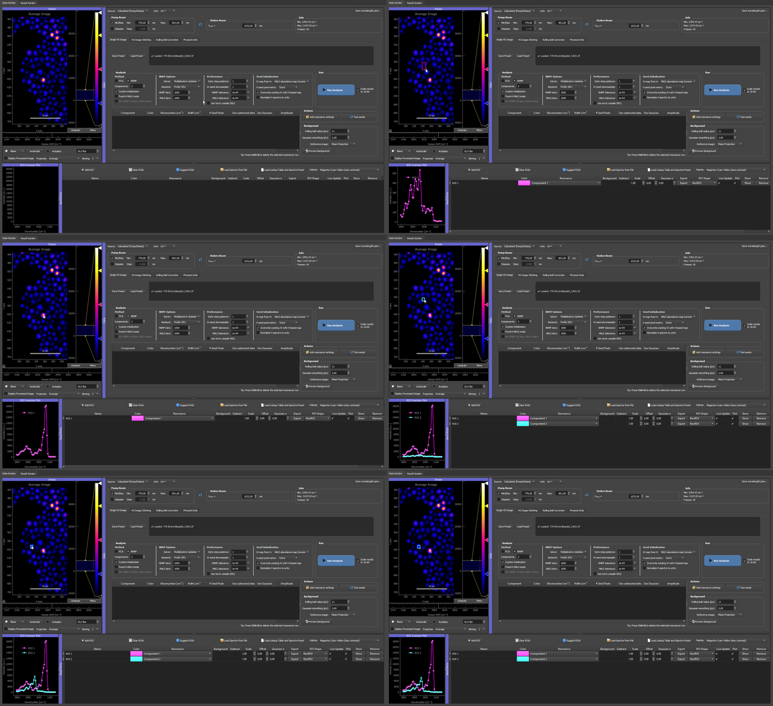 Demo of the ROI manager with a hyperspectral CARS microbead dataset.
What the ROI Manager controls
The ROI Manager connects four things:
- The image view, where spatial ROIs are drawn.
- The ROI table, where each row stores seed settings.
- The ROI average plot, where ROI spectra and model spectra are displayed.
- The analysis setup, where rows are converted into H seeds, W seeds, labels, colors, and background settings.

The selected ROI row links the table, image view, and ROI average plot. In the screenshot, ROI 2 is selected in the ROI table. The same user ROI is marked with a yellow selection frame in the image view, and its corresponding spectrum is visible in the ROI average plot. The row's color column still defines the component/result color; the yellow frame is only the current selection indicator.
The most important rule is:
component number in ROI Manager -> component index in analysis/result viewer
If a row is assigned to component 3, its spectrum, color, label, and optional W seed are treated as information for analysis component 3.
The component-number column is the single source of truth
Two ROIs assigned to component 1 are averaged together to build that component's H seed. A typo in the component number (e.g. assigning a background ROI to component 2 instead of 4) silently produces wrong seeds because nothing else in the UI cross-checks it. Glance at the component column whenever the analysis result surprises you — it is by far the most common preventable mistake.
Top buttons
The top buttons create or load ROI Manager entries.
Add ROI
Creates a new spatial ROI in the image view. The app asks for a component number and suggests the smallest unused component where possible. The ROI is added to the table and its mean spectrum can be used as an H seed.
Clear ROIs
Removes all ROI Manager rows and image ROIs. Use this when starting a new seed setup.
Suggest spectra / ROIs (VCA)
Estimates the pure component spectra directly from the data with Vertex Component Analysis and, by default, grows a real ROI around each component's purest pixel (the ROI's mean spectrum becomes the seed). With the Place ROIs option off, the endmember spectra are added as dummy ROI rows instead. The dialog also offers the number of endmembers (defaults to the analysis component count), the grow measure (cosine similarity / least-squares / selective score / NNLS abundance), and a maximum ROI half-size.
This is the recommended automatic seeding method. The full explanation is in Suggest spectra (VCA).
The older spatial-clustering Suggest ROIs method is now deprecated and no longer has its own button; it is reachable through a toggle inside the Suggest spectra (VCA) dialog. It still works, but VCA is generally more reliable; prefer the clustering method only for purely spatial detection. Its full settings dialog is explained in Suggest ROIs (clustering-based, legacy).
Existing ROIs are respected. Before candidate detection starts, every pixel already covered by a drawn ROI — whether placed manually or from a previous auto-suggestion run — is zeroed out in the response map. The algorithm is completely blind to those areas and will not place a new suggestion on top of an existing one. This means you can place a ROI manually on a known structure first and then run Suggest ROIs to fill in the remaining structures automatically without getting duplicates. Dummy spectrum rows and Gaussian model rows have no spatial footprint and are not masked.
Load Spectrum from File
Loads external spectra from CSV, TXT, or ASC files. Loaded spectra appear as dummy ROI rows because they carry spectral information without a drawn image ROI.
Load Lookup Table and Spectra Preset
Loads a result-viewer .preset file created from the result viewer with Save Histogram and Spectra Preset (see Save Histogram and Spectra Preset for the save side).

This is the canonical way to replay a finalised analysis on a new FOV of the same sample. The .preset carries the color scheme, the histogram levels, and the spectra used in the previous analysis. Loading it before running a new analysis means the next FOV starts from the same display state and the same spectral basis as the reference one, which is what makes results visually and quantitatively comparable across fields.
When the preset is loaded, the GUI asks how it should be applied:
LUTs Only: apply the saved component colors and histogram/LUT settings to the current result/component setup without importing new dummy ROI rows.LUTs + ROIs: also import the saved spectra as dummy ROI rows so they can be reused as H seeds.
Use LUTs Only when you already have the correct ROI/component setup and only want to reuse the visual style. Use LUTs + ROIs when the preset should also transfer spectral seeds into the ROI Manager.
Spectra loaded from a .preset enter the table as fixed dummy seeds — they do not depend on any drawn region in the current image. If the saved spectral axis differs from the axis of the currently loaded dataset, the spectra are interpolated (and extrapolated at the edges) onto the current axis, so the same .preset can be reused across acquisitions with slightly different spectral windows.
Palette
Switches the default component-color palette for the current session. Four palettes ship out of the box — the default magenta-cyan-yellow trio (best contrast on dark composites), a high-contrast magenta-green palette, the color-blind-safe Okabe-Ito palette, and a legacy classic-RGB cycle. See Default color palette in the results page for the full table of palettes and when to use each.
The same dropdown also appears in the result-viewer toolbar (next to Save Histogram and Spectra Preset). The two selectors are bidirectionally synced: picking a palette in one updates the other instantly, because both read from the shared component-color manager. The selection is persisted in the application JSON preset (Save Preset) and restored on load.
Per-component color edits override the palette. Clicking the color swatch in any ROI row's Color column (see Table columns below) opens a color picker. When the picked color differs from the palette's baseline value for that component, both Palette dropdowns append (customized) to the current entry, for example "Magenta–Cyan–Yellow (max contrast) (customized)", as a visual reminder that the visible color set has diverged from the palette default. The custom color itself is persisted in the application JSON preset alongside the palette name, so a customised palette round-trips through Save Preset / Load Preset correctly.
To restore the palette baseline (i.e. undo every per-component color edit in one click), re-select the same palette in the dropdown. Re-applying the active palette resets all component colors to their baseline values and clears the (customized) tag in both selectors.
Custom palettes can be added by editing the PALETTES and PALETTE_LABELS dictionaries in `hs_mosaic/widgets/color_manager.py. Your new palette then appears in both dropdowns automatically. See Adding a custom palette for the recipe.
Row types
The table can contain several kinds of rows.
Spatial ROI row
A real ROI drawn on the image. Its H seed is the mean spectrum of pixels inside the ROI.
Dummy spectrum row
A row without a visible ROI shape. It stores a spectrum from a CSV/TXT/ASC file, a result import, or a preset. It behaves like an H seed.
Gaussian/model row
A generated spectral model row. It stores a Gaussian seed spectrum for a component. It is useful when a component is expected at a known resonance or wavelength.
W-only row
A row that stores a fixed W seed but does not provide an H spectrum. This is used for fixed spatial maps, background components, or result-derived W seeds. These rows do not plot a fake H spectrum.
H+W result row
A row imported from a previous result that stores both the spectral component H and the spatial map W. This can be used to refine or transfer a previous decomposition.
Table columns
Name
The component/ROI label. This name is propagated to plots, result labels, and Fiji/ImageJ export labels where possible. Rename rows before final export.
Color
The component color. This controls ROI display, spectrum plot color, result component color, composite colors, and exported LUT colors. Click the swatch to open a color picker for that one component; the change is applied immediately to every widget that uses the color.
The initial value comes from the active Palette (see the Palette dropdown described under Top buttons). Picking a color that differs from the palette's baseline for that component tags the current palette as (customized) in both palette dropdowns; the custom color is saved with the application JSON preset. Re-selecting the same palette in the dropdown resets every component's color back to the palette baseline.
Resonance
This column is the component assignment. The label is historical. Selecting Component 3 means the row contributes to analysis component index 3.
Background
Marks the row as a background component. This is useful when a component should be interpreted or initialized as background rather than sample signal. The algorithm always assigns unsubtracted singal to the latter to minimize cross talk with components containing spcific information.
Subtract
Uses the row for background subtraction. Only use this intentionally, because subtraction changes the processed data passed to parts of the workflow.
Scale
Scales the displayed or prepared ROI spectrum. This is useful for matching seed amplitudes or visualizing spectra with different intensity ranges.
Offset
Adds an offset to the displayed or prepared ROI spectrum. This can help inspect spectra but should be used carefully for quantitative seed interpretation.
Gaussian sigma
Applies smoothing to the ROI spectrum. This can suppress noise in a seed spectrum, but excessive smoothing can remove real spectral structure.
Export
Exports the selected ROI/spectrum information where supported.
ROI Shape
Changes the shape of a real spatial ROI. Supported ROI shapes include line, rectangle, ellipse, and rotatable rectangle. Dummy rows do not have editable shapes.
Live Update
Controls whether the ROI spectrum updates while the ROI is moved/resized. Disable this for large data if interaction becomes slow.
Plot
Shows or hides the row in the ROI average plot. For W-only rows this can be disabled because no H spectrum should be plotted.
Show
Centers the image view on a spatial ROI. If the row stores a fixed W seed, this button becomes Show W and opens the W seed image.
Remove
Deletes the row and its associated ROI or dummy seed.
H seeds from spatial ROIs
For a spatial ROI, the H seed is the average spectrum of the pixels inside the ROI:
where \(R_i\) is the set of pixels inside the ROI assigned to component \(i\).
Implementation-shaped view:
pixels = pixels_inside_roi(row)
H0[component, :] = mean(X[pixels, :], axis=0)
Use this when the ROI contains a region that is visually dominated by one component.
Each spatial ROI row's H seed is exactly the mean spectrum above. With the row's Live Update column enabled, that mean is recomputed continuously while the ROI is dragged or resized, so the plotted seed follows the box in real time. Drag it onto the cleanest region for the component and watch the fingerprint settle. (Disable Live Update on very large stacks if interaction becomes slow.)
Multiple rows for one component
Several rows can point to the same component. This is useful when several regions represent the same material or when multiple seed sources should describe one component.
Practical interpretation:
- Multiple spatial ROIs for one component represent repeated observations of the same spectral class.
- Multiple fixed W rows for one component are averaged before analysis.
- Multiple labels/colors for the same component should be avoided; keep the final row names and colors consistent.
If two rows assigned to one component are actually different materials, increase the component number and separate them.
Dummy rows and loaded spectra
Loaded spectra and imported result spectra are stored as dummy ROIs. A dummy row has no spatial rectangle in the image, but it still appears in the table so it can be named, colored, assigned to a component, plotted, saved, and reused.
Dummy rows are the correct representation for:
- External spectra from CSV/TXT/ASC files.
- Spectra loaded from
.presetfiles whenLUTs + ROIsis selected. - Gaussian/model spectra.
- Result spectra imported back from the result viewer.
Fixed W seeds
A fixed W seed is a spatial map attached to a row. It defines where a component is expected spatially.
Fixed W seeds can come from:
- Imported result W maps.
- Rolling-ball/background components.
- H+W result imports.
If a row has a fixed W seed, the Show button becomes Show W.
Important limitation:
fixed W seed shape must match the current image shape
If new data are loaded or binning changes, old fixed W seeds may no longer match the image dimensions. The GUI removes incompatible fixed W seeds and warns the user.
ROI average plot
The ROI average plot shows spectra from plotted ROI Manager rows. It uses the current spectral axis:
- Wavenumber axis for Raman/CARS/SRS data.
- Wavelength axis for nm data.
- Channel labels for custom labeled data.
Gaussian/model curves can be shown as fallback curves for a component. If an ROI spectrum for that component is plotted, the model curve is hidden so the plot does not show two competing seed curves for the same component.
Clicking a ROI row selects the matching ROI object and makes it easier to connect the table entry with the plotted spectrum. This is useful when several ROIs overlap spatially or when several spectra are shown in the ROI average plot at once.
Background and subtraction
Background rows have two different meanings depending on the settings:
Backgroundmarks the row as a background-like component.Subtractuses the selected row for background subtraction.
These are not the same operation. A background component can be modeled during analysis, while subtraction changes the data before or during seed estimation.
Use subtraction only when you intentionally want to remove a measured background spectrum. Use a background component when the background level is relatively high.
Interaction with result viewer
The result viewer can import components back into the ROI Manager. The import can be:
- H only: stores the result spectrum as a dummy H seed.
- W only: stores the result map as a fixed W seed.
- H+W: stores both spectrum and map.
This is what makes the result viewer into a feedback loop on the seed setup:
run random NNMF
inspect result
import useful component into ROI Manager
rename/color/assign component
rerun seeded NNMF or fixed-H NNLS
What presets save
The main application preset saves ROI Manager state, including:
- Spatial ROI positions and sizes.
- Dummy spectra.
- Fixed W seeds.
- Component assignments.
- Names.
- Colors.
- Background/subtraction flags.
- Scale, offset, and smoothing settings.
- Plot/live-update state.
Gaussian model rows are regenerated from the resonance/spectral settings instead of being stored as normal ROI rows.
The result-viewer .preset is different:
- it stores result-viewer spectra, component colors, and histogram/LUT settings,
- it can be loaded as
LUTs OnlyorLUTs + ROIs, - it is useful for transferring a visual style or a seed spectrum set,
- it is not a full substitute for the main JSON application preset.
Recommended workflow
- Load data and set the spectral axis.
- Add or load seed rows.
- Assign component numbers.
- Rename rows with final biological/chemical labels.
- Set colors.
- Plot and inspect spectra.
- Check background/subtraction settings.
- Run analysis.
- Save the application preset.