Quickstart
This page walks through a minimal end-to-end analysis in roughly 10 minutes. It assumes the GUI can already start.
There are two supported ways to get to that point:
- Windows users who do not want Python can use the standalone Windows .exe, including the CUDA package for compatible NVIDIA GPUs.
- Users who want to run from source or manage their own environment can use the full Python installation.
What you need
- A 3D hyperspectral TIFF stack (channel, y, x).
- Optionally: a
wavelength.jsonfile in the same folder as the TIFF.
If you do not have real data yet, the Synthetic quickstart example shows how to generate a small test dataset from Python.
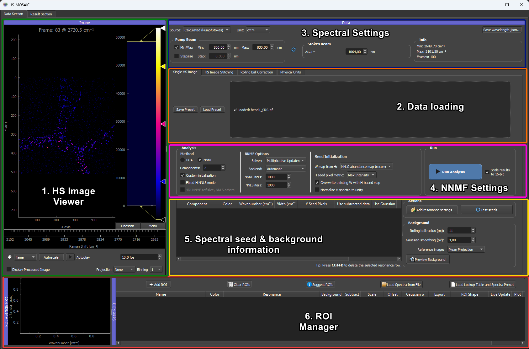
Overview of the main HS-MOSAIC window. The data viewer (top left), ROI Manager (bottom left), Analysis panel (top right) and result viewer (bottom right) are the four docks referenced in the steps below.
Minimal workflow at a glance
| Stage | GUI area | Main control |
|---|---|---|
| Load data | Single HS Image tab | Drag-and-drop area or click the drop area |
| Check axis | Spectral-axis widget | Calculated pump/Stokes or custom/manual axis |
| Define seeds | ROI Manager | Add ROI or Load Spectrum from File |
| Run seeded NNMF | Analysis panel | NNMF + Custom initialization + Run Analysis |
| Inspect/export | Result viewer | Composite Overview, Save H as CSV, Export Composite |
Step 1: Start the GUI
With the standalone Windows .exe, extract the whole portable zip and double-click the app:
HS_MOSAIC.exeinsideHS_MOSAIC_CPU_v...for the normal CPU package, orHS_MOSAIC.exeinsideHS_MOSAIC_GPU_CUDA..._v...for the PyTorch/CUDA package.
Keep the .exe next to its _internal folder.
With a full Python installation, install the package in an activated environment first:
pip install hs-mosaic                  # CPU-only
pip install "hs-mosaic[torch]"         # adds CPU PyTorch backends (not GPU)
# pip install -e .                     # editable install from a clone
Then launch the GUI:
hs-mosaic                    # console / shortcut launcher
python -m hs_mosaic          # equivalent module form
or on Windows:
hs-mosaic.bat
Step 2: Load the TIFF stack
In the Single HS Image tab, either:
- click the drop area and pick the TIFF from the file dialog, or
- drag and drop the TIFF file onto the drop area.
The GUI loads the stack and displays the first channel.
If a wavelength.json file is present in the same folder, the spectral axis is applied automatically. Otherwise, set the spectral axis manually in the spectral-axis widget (see Spectral axis and channel labels).
Step 3: Check the spectral axis
Scroll through the channel slider and check that the spectral axis numbers or labels make sense for your data. If they are wrong, correct the axis settings before continuing.
For CRS/CARS/SRS data, use the calculated pump/Stokes mode. For fluorescence data with known filter wavelengths, use the manual/custom axis mode.
Step 4: Add ROIs or seed spectra
Open the ROI Manager panel. Draw one or more ROIs on regions in the image that represent distinct chemical components:
- Click Add ROI in the ROI Manager.
- Move and resize the box to cover a region dominated by one component.
- Assign the ROI to a component number.
- Check the ROI average spectrum to confirm it looks representative.
Repeat for each expected component. If you have known reference spectra, use Load Spectrum to import them instead of drawing ROIs (see Loading custom seed spectra).
Seeds are the scientific decision
The quality of a seeded NNMF (or fixed-H NNLS) result is dominated by the seeds, not by the solver settings. Spend the time here: draw ROIs in genuinely spectrally distinct regions, sanity-check each ROI-averaged spectrum, and add a dedicated background ROI if the dataset has a slowly varying baseline. Defaults are correct for almost everything in the Analysis panel; the seeds are the part you defend.
Step 5: Run the analysis
In the Analysis panel:
- Set Number of components to match the number of ROIs or seeds.
- Select NNMF.
- Keep Custom initialization enabled. This is the seeded NNMF workflow.
- Leave Fixed-H NNLS mode disabled for the first run.
- Leave W map from H at NNLS abundance map (recommended) unless you have a reason to change it.
- Click Run Analysis.
The analysis runs in a background thread. A progress bar shows status. When it finishes, the result viewer opens.
To run fixed-H NNLS later, keep NNMF and Custom initialization enabled, enable Fixed-H NNLS mode, and make sure every component has an H seed.
Step 6: Inspect the result
In the result viewer:
- The Composite tab shows a false-color overlay of all component maps.
- The Channel tab shows one component map at a time.
- The spectral plot shows the fitted H spectra for each component.
Adjust histogram levels if maps look flat. Use the color picker to change component colors. Check whether the component spectra resemble the expected chemical signatures.
If the result looks wrong: - Go back to the ROI manager and adjust or add ROIs. - Try Fixed-H NNLS if the spectra look good but the maps are noisy. - Try PCA first to see the dominant variance patterns.
For guidance on choosing the right mode, see Analysis modes.
Step 7: Export
To export results:
- Save H as CSV: exports the component spectra to a text file.
- Export Composite: exports a Fiji/ImageJ-compatible multi-channel TIFF with LUTs and labels, or a rendered PNG.
Before exporting, set the physical pixel size in the Physical Units panel if scale-bar metadata is needed.
Step 8: Save a preset
Use Save Preset to save the full session state (ROIs, seeds, colors, analysis settings, histogram levels) to a JSON file. This lets you reproduce the analysis later or apply the same seed setup to a new dataset.
See Presets and reproducibility for details.
What next?
- Concepts: the unmixing model, what W and H mean, how seeds work.
- Analysis modes: when to use PCA, NNMF, or fixed-H NNLS.
- Seeds, spectra, and W maps: how to build better seeds.
- Physical units and rolling-ball correction: pixel size, scale bars, illumination correction.
- Results and export: full export workflow.