NNMF and NNLS modes

This page explains the multivariate modes used by the GUI from two angles at once:

• the intuitive picture needed to understand what the modes are doing,
• the mathematical model actually implemented by the software.

For the more workflow-oriented explanation, see 02 Analysis modes. Numbered citations like [5] resolve to the References section at the end of the page.

Why these modes are needed

Hyperspectral CRS, CARS, SRS, Raman, or fluorescence stacks are usually recorded as many grayscale slices across a spectral axis [16, 17]. Looking at dozens of slices one by one is slow and often misleading because the relevant information is spread across the whole stack.

The point of multivariate analysis here is not only dimensionality reduction in the abstract. It is a practical reorganization of the stack into a small set of spectral patterns, a matching set of spatial maps, and a false-color view that makes the dominant structures easier to inspect in one image. The raw stack is largely redundant or background-dominated; the analysis modes compress it into a smaller number of components that can be inspected as spectra and maps [14, 15].

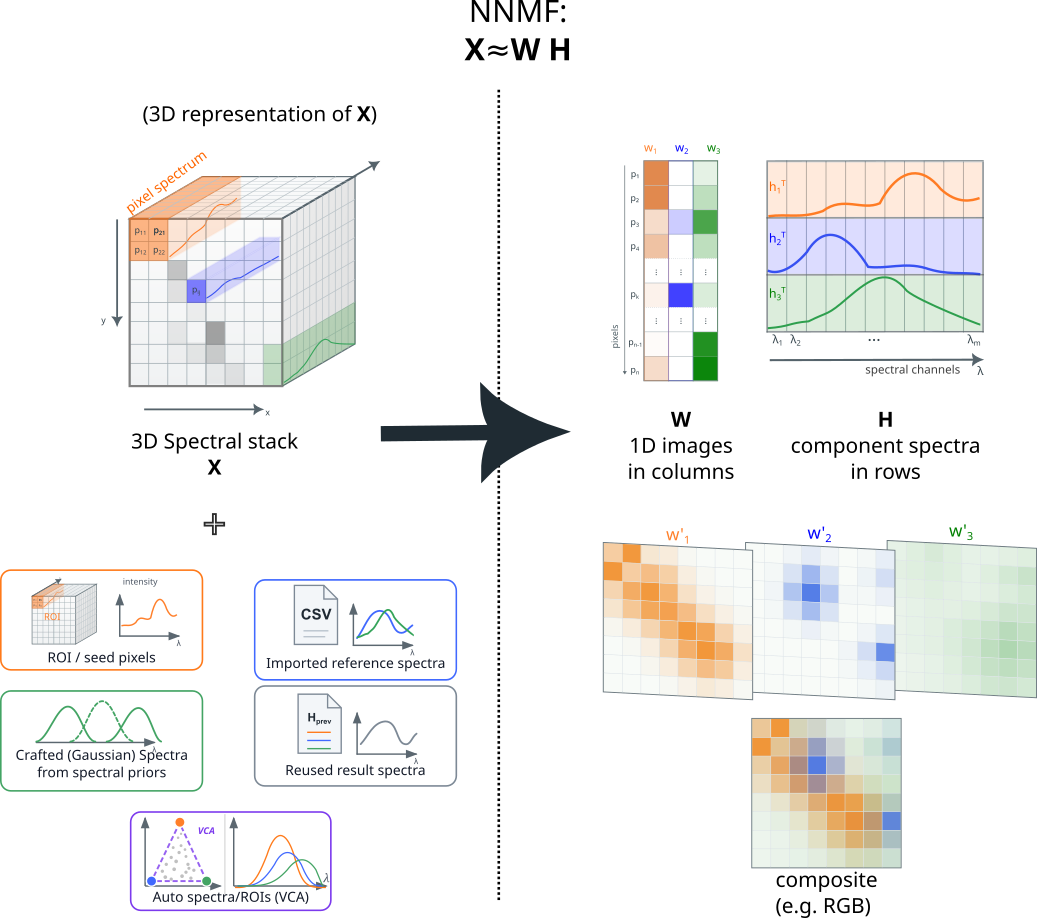
Data layout

The image stack is reshaped into a 2D data matrix

where each row is one pixel spectrum and each column is one spectral channel.

In the NNMF and NNLS-based modes, the target factorization is

with

• \(W \in \mathbb{R}_{\ge 0}^{n_\mathrm{pixels} \times n_\mathrm{components}}\): spatial maps or abundances,
• \(H \in \mathbb{R}_{\ge 0}^{n_\mathrm{components} \times n_\mathrm{channels}}\): component spectra.

This is the canonical NMF model [5, 8, 9]. In the GUI:

• each row of H is shown as a spectrum,
• each column of W is reshaped back into an image,
• the result viewer combines selected W maps into false-color composite images.

H carries spectral behavior, W carries where that behavior occurs spatially [14].

There is a component-wise scale ambiguity in NNMF [8, 9]: for any positive constant \(a\), replacing one component by \(a W_i\) and \(H_i / a\) leaves that component's contribution unchanged. This is why normalized generated W seeds are valid for seeded NNMF: both W and H remain free during fitting, so the optimizer can adapt the matching H row to the normalized W0 scale. The GUI uses this convention for seeded NNMF initialization — generated W0 maps are normalized to a comparable unit maximum, while H0 spectra keep the spectral/count scale from ROIs, files, Gaussian models, or seed pixels.

PCA

Intuition

PCA does not try to find chemically pure components. It asks a different question:

Along which spectral directions does the dataset vary the most?

Geometrically, PCA is a rotation of the coordinate system. Instead of describing each pixel by the original spectral channels, it creates new orthogonal axes — the principal components — that point along the strongest variance directions in the data [1, 2, 3].

The first principal component explains the largest variance, the second explains the largest remaining variance under the orthogonality constraint, and so on. PCA is useful for:

• fast inspection of an unknown dataset,
• detecting dominant gradients and correlations,
• estimating how many major patterns are present,
• spotting artifacts that affect many channels together.

Model

Before PCA, the GUI standardizes each spectral channel [3]:

It then estimates

where:

• P contains the principal component spectra (loadings),
• T contains the corresponding pixel scores.

This is the standard score–loading decomposition that traces back to Pearson [2] and is treated thoroughly in Jolliffe [3].

Interpretation in this project

PCA is often a very good first look, but it has important limitations for chemical interpretation:

• the components are orthogonal by construction, not chemically independent,
• negative values are allowed,
• one molecular signature can be split over several components,
• strong non-chemical correlations can dominate the leading components.

PCA often reveals the important resonances, but it can mix chemistry with gradients, split one resonance across several components, and produce signed outputs that are awkward to interpret physically [14]. Use PCA when you want a diagnostic or an initial estimate, not when you need strictly non-negative abundance-like maps.

Random NNMF

Intuition

NNMF replaces the PCA rotation picture with an additive mixing picture:

Each pixel spectrum is approximated as a non-negative sum of a few non-negative component spectra.

That is often easier to interpret for imaging data because intensities and abundances are naturally non-negative. The decomposition is described as parts-based [5, 7]: the model builds each pixel from additive contributions only, without sign cancellation.

Historically, this class of methods was used under the name positive matrix factorization [4] before Lee and Seung made it widely known [5, 6].

Model

Random NNMF solves

starting from unguided initial matrices [6, 9].

The result is exploratory:

• spectra and maps are both discovered from the data,
• no seed information is enforced,
• different initializations can lead to different local optima.

NMF with the Frobenius cost is non-convex jointly in W and H [8, 9]; only local minima are guaranteed. This is why initialization (seeded NNMF below) matters in practice.

Interpretation in this project

Random NNMF is useful when no reliable prior spectra exist yet. It is usually more physically intuitive than PCA because the result is additive and non-negative, but it is still not guaranteed to find the chemically preferred decomposition.

In practice it works best as:

• a first non-negative exploratory pass,
• a source of candidate result components that can later be imported back as seeds,
• a comparison point against seeded NNMF.

Seeded NNMF

Intuition

Seeded NNMF keeps the same non-negative matrix factorization model but starts from prior knowledge instead of random guesses. The question becomes:

If I already have a rough idea what some spectra or maps should look like, can the algorithm refine them while still adapting to the data?

This matters most for difficult CRS data: if resonances overlap strongly or the signal-to-background ratio is poor, unguided methods can mix components, but a seeded decomposition can be steered toward the desired clustering [14].

Model

The optimization target stays the same:

but the solver starts from user-guided seeds

and then updates both matrices. The seeds are not hard constraints — they are informed initial conditions:

Because the cost surface has many local minima [8, 9], the choice of W0 and H0 directly determines which one the solver converges to. That is the whole reason seeding helps on hard data.

What can become a seed

H0 can come from:

• ROI average spectra,
• imported spectra,
• Gaussian resonance models,
• previous result spectra,
• spectral information entered in the GUI.

W0 can come from:

• fixed W seeds,
• imported result maps,
• background maps,
• or from one of the H-driven W-seed estimation modes.

W-seed modes

If only a spectral seed is available, the GUI estimates W0 from the data and the current H0. The active W-seed mode decides how:

• nnls: coefficient maps from a non-negative least-squares fit,
• selective_score: a heuristic map based on target projection and competition against other seeded spectra,
• h_weighted: a legacy channel-weighted image heuristic,
• average: average image fallback,
• empty: almost neutral homogeneous fallback.

The important separation is:

• missing or incomplete H is discovered from the current basis through the residual-based seed logic,
• once a usable H exists, the final W seed for that component is built with the selected W-seed mode.

So the basis finding and the W-map construction are related, but they are not the same step.

Picking nnls vs selective_score

nnls is the most aggressive option: for every pixel it solves a full non-negative least-squares fit against all seeded spectra at once, so it pushes the decomposition toward maximum unmixing. Each pixel is explained by as few components as possible, and overlap is resolved by assigning the contribution to whichever seeded spectrum fits the residual best. This makes nnls the right default when components are expected to be spatially separable — different chemistries living in different pixels — and you want clean, near-binary abundance maps as the starting point for NNMF.

selective_score is the softer alternative. It still favors the target spectrum, but it down-weights pixels that also score well against competing seeded spectra, instead of forcing one winner per pixel. This makes it the right choice when mixing across pixels is physically expected — e.g. lipids and protein co-localized inside the same cell, or a fluorophore mixture inside a single voxel — and a pixel can legitimately carry several components at once. nnls in that situation tends to over-separate: pixels with a real mixture get assigned almost entirely to one component, which the subsequent NNMF then has to undo.

A simple rule of thumb:

• Components live in different pixels → nnls.
• Components share pixels by design → selective_score.
• You can't tell yet → try nnls first and inspect the W maps; if the maps look implausibly clean and disjoint compared to what you expect biologically, switch to selective_score for the seeding step.

This only affects the seed given to NNMF. The final fitted W after seeded NNMF can still recover mixed pixels because both W and H are updated during the fit — the choice mostly determines which local optimum the optimizer converges to.

Residual-based H seed fallback

When a component has no usable H0 spectrum, the GUI tries to estimate one from the residual that is not explained by the already seeded components:

1. Build a basis from the existing non-empty H0 rows.
2. Choose the component's working data. Background components use raw data. Other components use processed/background-subtracted data unless their Use subtracted data setting says to use raw data.
3. Solve a non-negative least-squares fit of the existing basis against each pixel spectrum.
4. Subtract that fitted signal from the working data and keep the positive residual.
5. Select strong residual pixels, optionally using the score-based metric to prefer spectra that are not already well described by the current basis.
6. Normalize candidate residual spectra by their own maxima, average them, smooth the average, and clamp it positive.
7. Rescale the new spectrum to the amplitude scale of the existing H0 basis where possible.

If this residual estimate is not usable, the older random smooth fallback is used. In fixed-H NNLS, this residual-filled H becomes part of the locked spectral basis, so it should be treated as an emergency fallback rather than as a trusted reference spectrum.

Spectral information and W overwrite

The Overwrite existing W with H-based map option controls whether W maps that came from spectral information are kept or replaced.

When overwrite is enabled and a component already has a valid H0, the spectral-info W image is not used as the final W0. The GUI rebuilds that component's spatial map from H0 with the selected W-seed mode. With the NNLS W-seed mode, this is an abundance map fitted from the fixed seed basis.

In that situation, spectral-info parameters such as resonance center, width, amplitude, and seed-pixel count usually do not shape the final W map. The main exception is the Use subtracted data flag, which can still choose raw versus processed/background-subtracted data for H-based W estimation and residual H-seed estimation. Spectral information can also still matter when it is used to create a missing H seed before the H-based W map is rebuilt.

Disable overwrite when the W image gathered from spectral information should remain the actual spatial seed.

Generated W0 maps are normalized per component before seeded NNMF starts. This includes NNLS abundance-map seeds and image-derived fallback seeds. The normalization is only an initialization convention: the NNMF solver can still rescale each W/H component pair during fitting because it updates both matrices.

Why seeded NNMF is often the most practical mode

Seeded NNMF is usually the most useful mode when you already know something about the sample, but do not want to freeze the spectral basis completely.

This is especially valuable when:

• two resonances overlap spectrally,
• background needs one or more dedicated components,
• some components are weak,
• you want the decomposition to follow known labels or ROIs,
• PCA or random NNMF gave only a rough first estimate.

This is also the mode where the GUI's custom seed logic matters most. It can take spectral priors, ROI averages, background information, and W-map hints and turn them into an initialization that is much more stable than random NNMF on difficult data.

Fixed-H NNLS

Intuition

Fixed-H NNLS is the strictest seeded mode. Once you trust the spectra, you stop asking the algorithm to discover new spectral shapes and ask only:

How much of each fixed spectrum is present in each pixel?

That is a pure abundance-fit problem. It is especially useful when you want stable spectra across slices, time points, or different fields of view.

Model

Fixed-H NNLS solves only for W:

For each pixel spectrum \(x_p\):

This is the classical non-negative least-squares problem, originally solved by the Lawson–Hanson active-set algorithm [10]. SciPy's nnls is a direct implementation [10]; the GUI's optional PyTorch backend uses projected gradient with FISTA acceleration instead [11, 12], which is significantly faster on GPU for large pixel counts. FISTA in its basic form is non-monotone and can oscillate on ill-conditioned problems; adaptive restart schemes that restore monotonicity and accelerate convergence are well established [13] and are a natural extension of the current backend.

Because H_seed is fixed, the fitted W in fixed-H NNLS is not just a seed-scale convention. The NNMF scale ambiguity is only harmless when both sides of a component pair can be rescaled together. In fixed-H NNLS, rescaling W alone changes \(W H_{\mathrm{seed}}\) and therefore changes the fit. Internally, these fixed-H NNLS coefficients should remain on their fitted scale rather than being normalized to unit maximum. Display and export scaling can still be applied afterward for visualization.

Interpretation in this project

This mode is ideal when:

• the reference spectra are already trusted,
• you want comparable abundance maps across z or time,
• you do not want the spectral basis to drift between slices,
• you want the most controlled seeded analysis.

In 4D workflows this is often the cleanest way to reuse one spectral basis and solve only for the changing spatial maps.

One practical consequence is important for image interpretation: fixed-H NNLS can be more accurate in the sense that each pixel is fitted very strictly against the trusted basis, but the displayed maps can look grainier or more speckled than NNMF maps. The false-color composite may therefore look less smooth even when the coefficient estimates are scientifically the more defensible result. In this project, visual smoothness and numerical faithfulness should not be confused automatically.

Solver-level numerical details

This section collects the implementation-level notes that affect reproducibility and how to compare results against other NMF/NNLS implementations.

Non-negativity, exact zeros, and the MU init eps lift

The NNMF constraint is

not strictly positive [5, 8, 9]. Exact zeros are valid in the data X, in the seeds W0 and H0, and in the fitted factors W and H. Zero entries simply mean "no contribution from this component at this pixel/channel". The GUI preserves zeros in the loaded image and in user-supplied seeds.

The only place this needs a caveat is the choice of NNMF solver. The GUI exposes two solvers via scikit-learn (mu, cd), with an optional PyTorch backend for mu.

• Multiplicative updates (mu). Each iteration multiplies the current W and H by a non-negative ratio [5, 6]:

$$ W \leftarrow W \odot \frac{X H^\top}{W H H^\top + \varepsilon}, \qquad H \leftarrow H \odot \frac{W^\top X}{W^\top W H + \varepsilon}. $$

An entry that is exactly zero at initialization stays zero forever, because every update multiplies it by zero. This zero-stuck-zero property is intrinsic to MU and has been noted since the original Lee–Seung derivation [5, 6, 9]. To avoid the trap, MU custom inits are lifted to >= eps (a small machine-scale constant) right at the solver boundary. The lift only touches the matrix that is handed to the solver; the analyzer's stored seed_W and seed_H and the loaded image data are not modified. During iteration MU can still drive entries down toward zero, so the final W and H are free to contain genuine zeros — the lift exists only to give MU a non-zero starting point from which to update.

• Coordinate descent (cd). Each entry is updated by an additive step that can move it off zero, so an exact zero at initialization is not a fixed point [8]. CD inits are passed to the solver unchanged.

• NNLS abundance fits (used by the nnls W-seed mode and by Fixed-H NNLS). These are additive projected-gradient or active-set solvers [10, 11], so they have no zero-stuck-zero issue. Zero abundances are valid results and are not lifted.

Practical consequence: a seed (W0 or H0) with legitimate zero entries is fine. The GUI's own seed builders still emit strictly positive seeds because they are designed for MU initialization, but a user-provided seed that contains zeros — for instance an externally computed abundance map, or an H spectrum with truly silent spectral channels — is accepted as-is and only lifted internally if MU is the selected solver. CD and NNLS see the seed exactly as you provided it.

Convergence criteria

The iterative solvers stop when either a relative-improvement criterion is met or an iteration budget is exhausted. The exact criterion depends on which backend is used.

NNMF — multiplicative updates (PyTorch backend)

After each iteration the Frobenius reconstruction error is not computed: that would force a GPU↔CPU synchronization on every step. Instead the error is sampled every track_error_every iterations (default 10). Letting \(E_k\) denote the residual at the \(k\)-th sampled iteration,

the solver stops at the first sampled iteration where

with default tol = 1e-4 and default max_iter = 1000. This compares against the previous sample, not the previous iteration, so tol = 1e-4 here means "≤ 0.01 % relative improvement across a 10-iteration window", which is a slightly stricter test than the same tol interpreted per-iteration. If you compare convergence behavior against another implementation, this is worth keeping in mind.

NNMF — scikit-learn backend (mu and cd)

The scikit-learn backend uses its own internal stopping rule, parameterized by tol (default 1e-4) and max_iter (default 1000). The criterion is documented in sklearn.decomposition.NMF; the GUI does not modify it. Reported n_iter values are therefore not directly comparable between the PyTorch-MU and scikit-learn paths for the same tol.

NNLS — PyTorch FISTA backend

Each pixel chunk is solved with projected gradient + FISTA acceleration [11, 12]. Convergence is checked every 10 iterations:

with default tol = 1e-4 and default max_iter = 1000. Chunks that fail to meet the criterion within the iteration budget return their last iterate; the fit summary reports the per-chunk iteration counts and the maximum across chunks so non-convergence is visible.

NNLS — SciPy backend

The SciPy backend uses scipy.optimize.nnls, the Lawson–Hanson active-set algorithm [10]. It has no tol parameter — only an iteration limit (max_iter, default 1000). It either reaches the exact KKT optimum within the budget or returns the best iterate found.

Practical recommendation

For publication-grade runs:

• Start with the defaults (tol = 1e-4, max_iter = 1000).
• Inspect the fit summary after the analysis. If n_iter is at the cap or max_chunk_iter equals max_iter for NNLS, raise max_iter and re-run; the result was iteration-limited, not tolerance-limited.
• Tighten tol only when the reconstruction error is still visibly decreasing at the iteration cap.

Practical choice

The modes are best viewed as a progression of prior knowledge:

• PCA: discover variance directions.
• Random NNMF: discover non-negative additive components.
• Seeded NNMF: guide the decomposition but still let spectra adapt.
• Fixed-H NNLS: keep spectra fixed and solve only abundances.

For difficult CARS data, the practical conclusion from the thesis [14] still holds up well:

• PCA and random NNMF are very useful first passes,
• seeded NNMF is usually the strongest general-purpose mode when prior information exists,
• fixed-H NNLS is the most stable mode once the spectral basis is considered trustworthy.

References

References are numbered continuously; the topical headings below are visual groupings only.

PCA

1. Ali Cinar, Ahmet Palazoglu, and Ferhan Kayihan, Chemical Process Performance Evaluation, CRC Press, 2019. Geometric and covariance-based interpretation of PCA.
2. Karl Pearson, "On lines and planes of closest fit to systems of points in space," Philosophical Magazine 2(11), 559–572, 1901. Historical origin of PCA.
3. Ian T. Jolliffe, Principal Component Analysis, 2nd ed., Springer, 2002. Canonical PCA reference including the channel-standardization step.

NMF — model and algorithms

1. Pentti Paatero and Unto Tapper, "Positive matrix factorization: a non-negative factor model with optimal utilization of error estimates of data values," Environmetrics 5(2), 111–126, 1994. The earlier positive matrix factorization formulation.
2. Daniel D. Lee and H. Sebastian Seung, "Learning the parts of objects by non-negative matrix factorization," Nature 401(6755), 788–791, 1999. Canonical NMF model with the parts-based interpretation.
3. Daniel D. Lee and H. Sebastian Seung, "Algorithms for Non-negative Matrix Factorization," Advances in Neural Information Processing Systems 13, 556–562, 2001. Derivation of the multiplicative-update rules used by the MU solver.
4. Jean-Philippe Brunet, Pablo Tamayo, Todd R. Golub, and Jill P. Mesirov, "Metagenes and molecular pattern discovery using matrix factorization," PNAS 101(12), 4164–4169, 2004. Parts-based and clustering-oriented interpretation of NMF.
5. Andrzej Cichocki and Anh-Huy Phan, "Fast local algorithms for large scale nonnegative matrix and tensor factorizations," IEICE Transactions on Fundamentals E92-A(3), 708–721, 2009. Coordinate-descent NMF algorithms referenced by sklearn.decomposition.NMF for the cd solver; covers local-minima behavior of the Frobenius cost.
6. Nicolas Gillis, "The why and how of nonnegative matrix factorization," in Regularization, Optimization, Kernels, and Support Vector Machines, Chapman & Hall/CRC, 257–291, 2014. Modern survey of NMF algorithms, identifiability, and the local-minima structure of the Frobenius cost.

NNLS — algorithms

1. Charles L. Lawson and Richard J. Hanson, Solving Least Squares Problems, Prentice-Hall, 1974 (reprinted as SIAM Classics in Applied Mathematics 15, 1995). The active-set NNLS algorithm used by SciPy's nnls.
2. Chih-Jen Lin, "Projected gradient methods for non-negative matrix factorization," Neural Computation 19(10), 2756–2779, 2007. Projected-gradient analysis of NMF subproblems, including the NNLS step solved by the PyTorch backend.
3. Amir Beck and Marc Teboulle, "A fast iterative shrinkage-thresholding algorithm for linear inverse problems," SIAM Journal on Imaging Sciences 2(1), 183–202, 2009. FISTA acceleration used by the PyTorch NNLS backend.
4. Brendan O'Donoghue and Emmanuel Candès, "Adaptive Restart for Accelerated Gradient Schemes," Foundations of Computational Mathematics 15(3), 715–732, 2015. Adaptive-restart variant of FISTA that restores monotonic convergence on ill-conditioned problems; cited as a natural extension of the current backend.

CRS imaging context

1. Christian Pilger, Development of novel Optics and Analysis Tools for enhancing Biomedical Imaging by Coherent Raman Scattering, PhD thesis, University of Bielefeld, 2019. Group-specific CRS and analysis context, including the seeded-NNMF reasoning.
2. Paul Greife, Implementation of a Hyper-Spectral Image Scan Capability in a Coherent Anti-Stokes Raman Scattering (CARS) Microscope, Master's thesis, University of Bielefeld, 2017. Project-specific image-stack reshaping and acquisition context.
3. Branko Vukosavljevic et al., "Vibrational spectroscopic imaging and live cell video microscopy for studying differentiation of primary human alveolar epithelial cells," Journal of Biophotonics 12(6), e201800052, 2019. Example application of CRS imaging with biologically meaningful spectral separation.
4. Chaoyang Zhang, Delong Zhang, and Ji-Xin Cheng, "Coherent Raman Scattering Microscopy in Biology and Medicine," Annual Review of Biomedical Engineering 17, 415–445, 2015. Broader motivation for CRS imaging in biological and clinical settings.